Original topic illustration: ChainView BTC866 original topic diagram · ChainView BTC866 Editorial · CC BY 4.0
Use information available at the time
A decision dated January cannot use a metric revised in March. Publication, retrieval and effective dates may differ. Today's completed history is not automatically the dataset an investor could have accessed then, and selecting early winners from a later ranking leaks information.
Preserving the first published version helps prevent revised future data entering an earlier signal. On-chain inputs also depend on confirmation and reorganisation. If a rule uses unfinalised blocks, describe what was observable then; a complete explorer history today does not prove an equally complete real-time feed existed.
A historical simulation is only as credible as its data availability assumptions; using a later revised metric at an earlier decision time leaks future information.
Keep failed assets in view
A universe containing only currently traded tokens excludes failures and delistings. Reconstruct eligibility at each historical point and state how exits are valued. Missing prices should not imply a free sale at the last quote; disclose the unresolved loss and data limitations.
Include assets that were tradable at the time even if they later failed. Missing-price assumptions can determine the result. If only surviving assets are available, limit the conclusion to that sample rather than reporting a market-wide return. Data expense and unavailability are themselves practical constraints on a strategy.
Including only coins or venues that still exist omits failures and delistings, creating survivorship bias in the investment universe.
Model execution friction
Fees, spreads, size, latency and depth affect outcomes. A signal calculated at the closing price may not be executable at that same price. Transfers between venues take time. Compare cost assumptions rather than publishing only the most flattering simulated equity curve.
Simulated order size must fit available depth; a large strategy cannot consume all historical volume for free. Fee tiers, rebates and borrowing need plausible historical assumptions. Today's best tier should not be applied retrospectively without justification. A sensitivity range is more informative than attractive precision several decimals beyond the data's reliability.
Model fees, spreads, order size, execution latency and unavailable liquidity, then separate model selection from genuinely out-of-sample evaluation.
Separate model selection from evaluation
Parameter fitting and out-of-sample testing must remain distinct. Trying many rules and reporting only the winner adds selection bias. Record the search range and unsuccessful alternatives. A later market change calls for renewed evaluation, not endless rewriting of historical rules.
Training, validation and final evaluation sets have distinct jobs. Repeatedly checking the final result and altering rules means it is no longer genuinely unseen. Preserve an experiment log and decision dates so others can assess selection bias rather than hiding repeated historical fitting behind sophisticated terminology.
Disclose parameter trials and fragile assumptions; a smooth backtest curve is not evidence that future returns are attainable.
Report what the experiment establishes
Document dataset versions, universe rules, trade timing, costs and missing values. A profitable historical simulation does not guarantee future execution or profit. Readers abroad also face currency and eligibility constraints; a backtest is a conditional research result rather than an instruction to commit funds.
The final note should include risks the model cannot represent well, such as outages, withdrawal delays and disappearing markets. Difficulty estimating extreme events is not a reason to omit them. A backtest can generate questions, while a real-money decision still requires independent assessment and a tolerable loss budget.
One useful robustness check delays the simulated trade by an additional interval and increases estimated execution costs. If the result disappears immediately, report that sensitivity rather than hiding the alternative. Another is to test a different historical subperiod without retuning. Neither exercise proves a strategy will work, but both can expose dependence on unrealistically precise timing or one favourable market episode that dominates the published aggregate return.
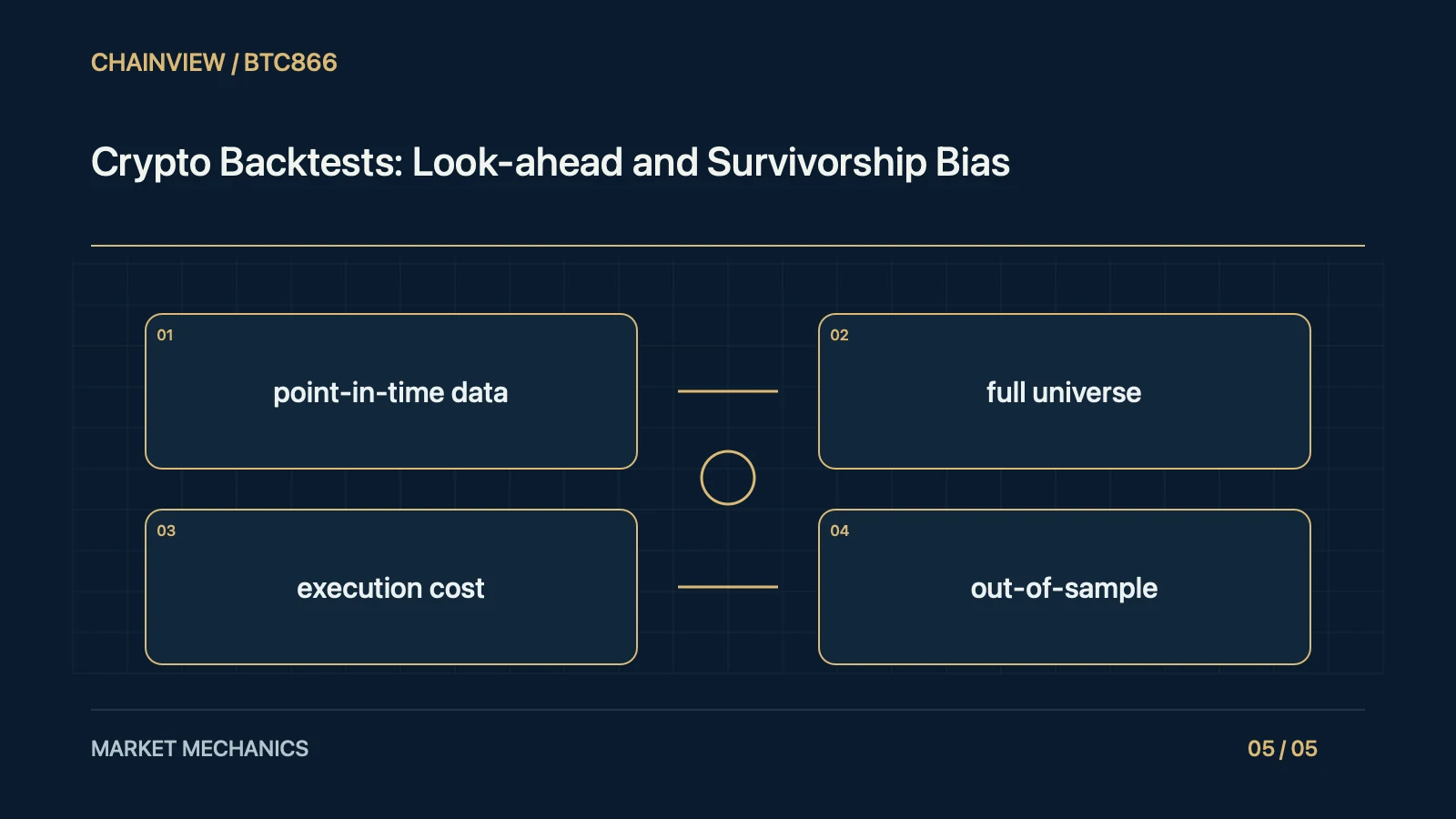
A useful worksheet for this topic has separate entries for point-in-time data, full universe, execution cost and out-of-sample. Fix one set of fictional inputs, change one condition at a time and identify which conclusion moves. Retain units, observation time and source beside every number. An unknown input should remain unknown rather than becoming zero by default. The purpose is to expose methodological dependence, not select the most flattering outcome. Before using the result for a real-money decision, compare its assumptions with actual fees, available liquidity, household spending needs and the loss the user can afford. A clean calculation cannot remove those constraints.